Show the code
library(sf)
library(tidyverse)
library(tmap)
library(here)
library(kableExtra)
library(usethis)
library(stars)
library(terra)
library(patchwork)library(sf)
library(tidyverse)
library(tmap)
library(here)
library(kableExtra)
library(usethis)
library(stars)
library(terra)
library(patchwork)# Create a list of all images that have the extension .tif and contain "sst"
sst_data <- list.files(here("posts", "prioritize_aquaculture", "data"),
pattern = "sst",
full.names = TRUE)
# Create a raster stack
sst <- c(rast(sst_data))
# Bathymetry
depth <- rast(here("posts", "prioritize_aquaculture","data", "depth.tif"))
# Exclusive Economic Zones
eez <- read_sf(here("posts", "prioritize_aquaculture","data", "wc_regions_clean.shp"))st_crs(eez) == st_crs(depth)[1] TRUEst_crs(eez) == st_crs(sst)[1] FALSEst_crs(sst) == st_crs(depth)[1] FALSEsst <- project(sst, crs(depth))# Create a named list of CRS comparisons
df_crs_comparisons <- list(
"sst vs depth" = st_crs(sst) == st_crs(depth),
"depth vs eez" = st_crs(depth) == st_crs(eez)
)
# Identify mismatched CRS comparisons
false_comparisons <- names(df_crs_comparisons)[!unlist(df_crs_comparisons)]
# Print results or display warning
if (length(false_comparisons) == 0) {
print("All CRS match.")
} else {
warning(paste(false_comparisons, collapse = "; "), " CRS projections do not match.")
}[1] "All CRS match."# Find mean SST from 2008-2012 and make one raster
sst_mean <- app(sst, fun = mean, na.rm = TRUE)
# Convert average SST from Kelvin to Celsius
sst_celsius <- sst_mean - 273.15
# Crop depth raster to match extent of SST raster
depth_crop <- crop(depth, sst_celsius)
depth_resample <- resample(depth_crop, y = sst_celsius, method = "near")
# Set CRS the same
depth_resample <- project(depth_resample, crs(sst))
# Check that depth and SST match in resolution, extent and CRS
if (identical(terra::res(depth_resample), terra::res(sst_celsius))) {
print("resolutions match")
} else {
print("resolutions don't match")
}[1] "resolutions match"if (identical(terra::crs(depth_resample), terra::crs(sst_celsius))) {
print("crs match")
} else {
print("crs don't match")
}[1] "crs match"if ((terra::ext(depth_resample) == terra::ext(sst_celsius))) {
print("ext match")
} else {
print("ext don't match")
}[1] "ext match"# Stack sst_celsius and resampled depth
sst_depth <- c(sst_celsius, depth_resample)Oysters require: - sea surface temperature: 11-30°C - depth: 0-70 meters below sea level
# Look at values
summary(sst_celsius)
mean
Min. : 7.02
1st Qu.:12.39
Median :14.07
Mean :14.16
3rd Qu.:16.06
Max. :32.72
NA's :41907 summary(depth_resample) depth
Min. :-5468
1st Qu.:-4023
Median :-1703
Mean :-1487
3rd Qu.: 881
Max. : 4112 # Create sst reclassification matrix for sst
rcl_sst <- matrix(c(-Inf, 11, NA, # min sst
11, 30, 1,
30, Inf, NA), # max sst
ncol = 3, byrow = TRUE)
# Use reclassification matrix to reclassify sst raster
reclass_sst <- classify(sst_celsius, rcl = rcl_sst)
# Create depth reclassification matrix
rcl_depth <- matrix(c(-Inf, -70, NA, # min depth
-70, 0, 1,
0, Inf, NA), # max depth
ncol = 3, byrow = TRUE)
# Use reclassification matrix to reclassify depth raster
reclass_depth <- classify(depth_resample, rcl = rcl_depth)
# Check that it worked
summary(reclass_sst) mean
Min. :1
1st Qu.:1
Median :1
Mean :1
3rd Qu.:1
Max. :1
NA's :46153 summary(reclass_depth) depth
Min. :1
1st Qu.:1
Median :1
Mean :1
3rd Qu.:1
Max. :1
NA's :98798 # Perform the operation: Both cells equal to 1
suit_loc <- (reclass_sst*reclass_depth)# Find area of suitable cells
suit_area <- cellSize(x = suit_loc, # locations suitable
mask = TRUE, # keeps NA
unit = 'km')
# Rasterize EEZ data
eez_raster <- rasterize(eez,
suit_area,
field = 'rgn')
# Use zonal algebra to sum the suitable area by region
eez_suitable <- zonal(x = suit_area,
z = eez_raster, # Raster representing zones
fun = 'sum',
na.rm = TRUE)
# To map our eez area with geometry later on
eez <- left_join(eez, eez_suitable, by = "rgn")# View the area per region of suitable habitat for Oysters
kable(eez_suitable, digits = 2,
caption = "Total Suitable Area for Oysters by Exclusive Economic Zone",
col.names = c("EEZ Region", "Area (km^2)"))| EEZ Region | Area (km^2) |
|---|---|
| Central California | 4939.80 |
| Northern California | 438.15 |
| Oregon | 1533.07 |
| Southern California | 3811.80 |
| Washington | 3224.69 |
# Plot regions and suitable areas together
tm_shape(depth) +
tm_raster(palette = "-Blues",
title = "Bathymetry\n(m above/below sea level)",
midpoint = 0,
legend.show = TRUE) +
tm_shape(eez) +
tm_polygons(fill = "area",
palette = "YlGn",
alpha = 0.65,
lwd = 0.2,
title = expression("Suitable habitat area (km"^2*")")) +
tm_text("rgn", size = 0.45) +
tm_compass(size = 1,
position = c("left", "top")) +
tm_scale_bar(position = c("right", "top")) +
tm_layout(legend.outside = TRUE,
frame = TRUE,
main.title = "Suitable Habitats for Oysters by \nWest Coast Exclusive Economic Zones")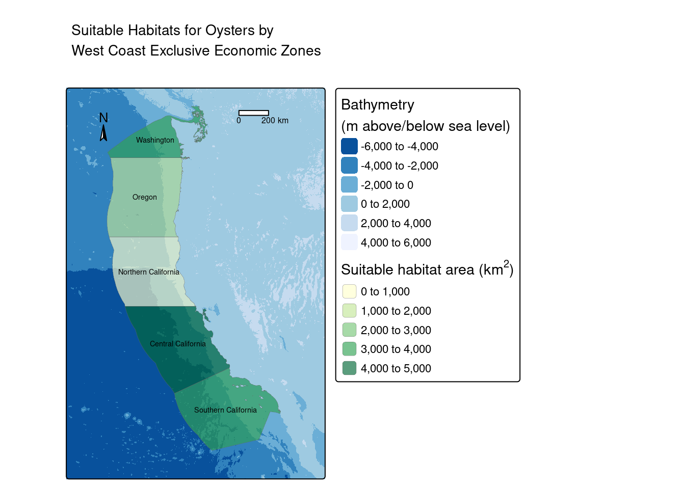
aquaculture_function <- function(species, min_sst, max_sst,
min_depth, max_depth) {
# Create a list of all images that have the extension .tif and contain "sst"
sst_data <- list.files(here("posts", "prioritize_aquaculture","data"),
pattern = "sst",
full.names = TRUE)
# Create a raster stack
sst <- c(rast(sst_data))
# Bathymetry
depth <- rast(here("posts", "prioritize_aquaculture","data", "depth.tif"))
# Exclusive Economic Zones
eez <- read_sf(here("posts", "prioritize_aquaculture","data", "wc_regions_clean.shp"))
# Match crs
sst <- project(sst, crs(depth))
# Find mean SST from 2008-2012 and make one raster
sst_mean <- app(sst, fun = mean, na.rm = TRUE)
# Convert average SST from Kelvin to Celsius
sst_celsius <- sst_mean - 273.15
# Crop depth raster to match extent of SST raster
depth_crop <- crop(depth, sst_celsius)
depth_resample <- resample(depth_crop, y = sst_celsius, method = "near")
# Set CRS the same
depth_resample <- project(depth_resample, crs(sst))
# Create sst reclassification matrix for sst
rcl_sst <- matrix(c(-Inf, min_sst, NA, # min sst
min_sst, max_sst, 1,
max_sst, Inf, NA), # max sst
ncol = 3, byrow = TRUE)
# Use reclassification matrix to reclassify sst raster
reclass_sst <- classify(sst_celsius, rcl = rcl_sst)
# Create depth reclassification matrix
rcl_depth <- matrix(c(-Inf, min_depth, NA, # min depth
min_depth, max_depth, 1,
max_depth, Inf, NA), # max depth
ncol = 3, byrow = TRUE)
# Use reclassification matrix to reclassify depth raster
reclass_depth <- classify(depth_resample, rcl = rcl_depth)
# Perform the operation: Both cells equal to 1
suit_loc <- (reclass_sst*reclass_depth)
# Find area of suitable cells
suit_area <- cellSize(x = suit_loc, # locations suitable
                          mask = TRUE, # keeps NA
                          unit = 'km')

# Rasterize EEZ data
eez_raster <- rasterize(eez,
                        suit_area,
                        field = 'rgn')

# Use zonal algebra to sum the suitable area by region
eez_suitable <- zonal(x = suit_area,
                      z = eez_raster, # Raster representing zones
                      fun = 'sum',
                      na.rm = TRUE)

# To map our eez area with geometry later on
eez <- left_join(eez, eez_suitable, by = "rgn")
# Map of suitable areas
map <- tm_shape(depth) +
tm_raster(palette = "-Blues",
title = "Bathymetry\n(m above/below sea level)",
midpoint = 0,
legend.show = TRUE) +
tm_shape(eez) +
tm_polygons(fill = "area",
palette = "YlGn",
alpha = 0.65,
lwd = 0.2,
title = expression("Suitable habitat area (km"^2*")")) +
tm_text("rgn", size = 0.45) +
tm_compass(size = 1,
position = c("left", "top")) +
tm_scale_bar(position = c("right", "top")) +
tm_layout(legend.outside = TRUE,
frame = TRUE,
main.title = paste("Suitable Habitats for", species, "by \nWest Coast Exclusive Economic Zones"))
# Print map
return(map)
}Red Abalone require: - sea surface temperature: 8-18°C - depth: 0-24 meters below sea level
aquaculture_function(species = "Red Abalone",
                     min_sst = 8,
                     max_sst = 18,
                     min_depth = -24,
                     max_depth = 0)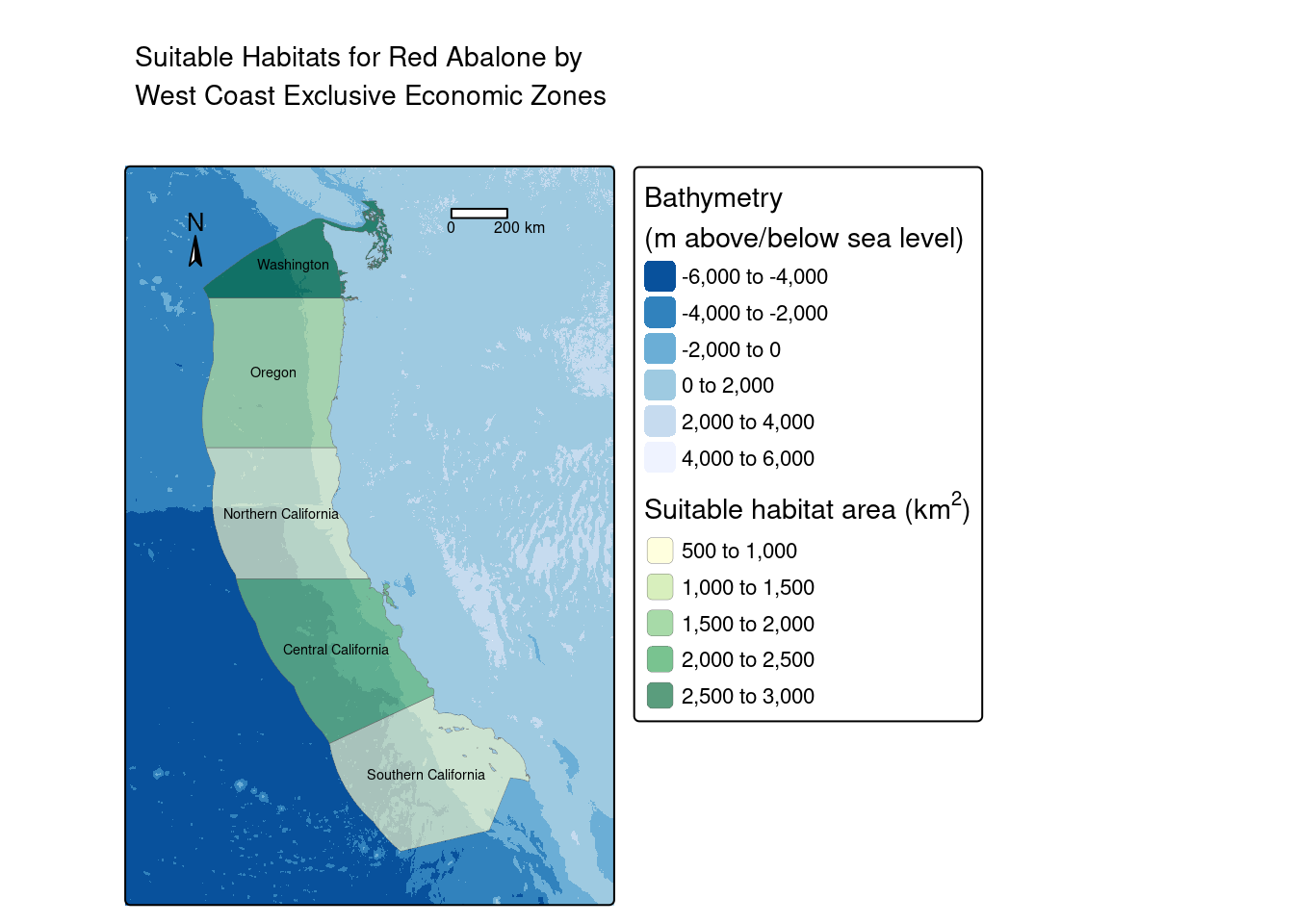
| Data | Citation | Link |
|---|---|---|
| SeaLife | Palomares, M.L.D. and D. Pauly. Editors. 2024. SeaLifeBase. World Wide Web electronic publication. www.sealifebase.org, version (08/2024) | [SeaLife (Red Abalone)](https://www.sealifebase.ca/summary/Haliotis-rufescens.html) |
| Bathymetry | General Bathymetric Chart of the Oceans. (n.d.). Gridded bathymetry data (general bathymetric chart of the oceans). GEBCO. https://www.gebco.net/data_and_products/gridded_bathymetry_data/#area | [Gridded Bathymetry Data](https://www.gebco.net/data_and_products/gridded_bathymetry_data/#area) |
| Sea Surface Temperature | NOAA Coral Reef Watch. 2019, updated daily. NOAA Coral Reef Watch Version 3.1 Daily 5km Satellite Regional Virtual Station Time Series Data for Southeast Florida, Mar. 12, 2013-Mar. 11, 2014. College Park, Maryland, USA: NOAA Coral Reef Watch. Data set accessed 2020-02-05 at https://coralreefwatch.noaa.gov/product/vs/data.php. | [NOAA’s 5km Daily Global Satellite Sea Surface Temperature Anomaly v3.1](https://coralreefwatch.noaa.gov/product/5km/index_5km_ssta.php) |
| Economic Exclusive Zones | Marine regions. (n.d.). https://www.marineregions.org/eez.php | [Marineregions.org](https://www.marineregions.org/eez.php) |
@online{wong2024,
  author = {Wong, Kimmy},
  title = {Prioritizing {Potential} {Aquaculture}},
  date = {2024-12-07},
  url = {https://kimberleewong.github.io/posts/prioritize_aquaculture/prioritizing_potential_aquaculture_blog.html},
  langid = {en}
}